Fernando Garcia

Home Research Blog Other About me

PHYS405 - Electricity & Magnetism I

Spring 2024

Problem 4.22

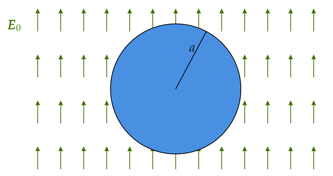
A very long cylinder of linear dielectric material is placed in an otherwise uniform electric field $E_{0}$ .

Find the resulting field within the cylinder.

(The radius is $a$ , the susceptibility $χ_{e}$ , and the axis is perpendicular to $E_{0}$ ).

Notie the uniformity of the field. Suppose it points in the $\hat{x}$ direction. The picture below shows a cross-section of the cylinder and the background $E_{0}$ field.

If we find the potential, we can find the field.

We will have to solve Laplace's equation. To do so, let's first write down the relevant boundary conditions:

Boundary conditions

(BC1) At $s = a$ , we have

ϵ \frac{\partial V_{in}}{\partial s} = ϵ_{0} \frac{\partial V_{out}}{\partial s}

(BC2) At $s = a$ again, we have

V_{in} = V_{out}

(BC3) When $s$ is much larger than $a$ , we should only experience a contribution from the external (uniform) field. We know what the field is. We see that

V_{out} \approx - E_{0} s \cos (ϕ)

Where $ϕ$ will be measured from the direction of the uniform $E_{0}$ field. Notice that this physically means that we can move perpendicularly to the field.

Solving Laplace's

Let's recall the general solution to Laplace's equation in Cylindrical coordinates (with $z$ -symmetry):

V (s, ϕ) = a_{0} + b_{0} \ln s + \sum_{k = 1}^{\infty} (s^{k} [a_{k} \cos (k ϕ) + b_{k} \sin (k ϕ)] + s^{- k} [c_{k} \cos (k ϕ) + d_{k} \sin (k ϕ)])

Inside: The $s^{- k}$ terms must go away, or the potential will explode. The same holds for the log term. We can safely ignore the constant term. We now have a cleaner expression:

V_{in} = \sum_{k = 1}^{\infty} s^{k} (a_{k} \cos (k ϕ) + b_{k} \sin (k ϕ))

Outside: The $s^{k}$ terms must go away, as well as the log term. Both of them will explode as $s \to \infty$ . The constant term here will make use of the third boundary condition, since $s >> a$ implies $s \to \infty$ and at this point we can ignore all the $s^{- k}$ terms.

V_{out} = - E_{0} s \cos (ϕ) + \sum_{k = 1}^{\infty} s^{- k} (c_{k} \cos (k ϕ) + d_{k} \sin (k ϕ))

The continuity condition (BC2) implies

\sum_{k = 1}^{\infty} s^{k} (a_{k} \cos (k ϕ) + b_{k} \sin (k ϕ)) |_{s = a} = - E_{0} s \cos (ϕ) + \sum_{k = 1}^{\infty} s^{- k} (c_{k} \cos (k ϕ) + d_{k} \sin (k ϕ)) |_{s = a}

Evaluated at $s = a$ , that is:

\sum_{k = 1}^{\infty} a^{k} (a_{k} \cos (k ϕ) + b_{k} \sin (k ϕ)) = - E_{0} a \cos (ϕ) + \sum_{k = 1}^{\infty} a^{- k} (c_{k} \cos (k ϕ) + d_{k} \sin (k ϕ))

While continuity of the derivatives (BC1) implies

ϵ \sum_{k = 1}^{\infty} k s^{k - 1} (a_{k} \cos (k ϕ) + b_{k} \sin (k ϕ)) |_{s = a} = [- E_{0} \cos (ϕ) - \sum_{k = 1}^{\infty} k s^{- k - 1} (c_{k} \cos (k ϕ) + d_{k} \sin (k ϕ))] ϵ_{0} |_{s = a}

Evaluated at $s = a$ , that is:

ϵ_{r} \sum_{k = 1}^{\infty} k a^{k - 1} (a_{k} \cos (k ϕ) + b_{k} \sin (k ϕ)) = - E_{0} \cos (ϕ) - \sum_{k = 1}^{\infty} k a^{- k - 1} (c_{k} \cos (k ϕ) + d_{k} \sin (k ϕ))

Where I used $ϵ_{r}$ rather than $ϵ, ϵ_{0}$ separately. The only coefficients that will remain are $a_{1}$ and $c_{1}$ .

We get two relations between $a_{1}$ and $c_{1}$ , each from each of the first two boundary conditions. We get the following (linear) system:

\begin{aligned} E_{0} & = - ϵ_{r} a_{1} - a^{- 2} c_{1} \\ E_{0} a & = - a a_{1} + a^{- 1} c_{1} \end{aligned}

That is:

(\begin{matrix} E_{0} \\ E_{0} a \end{matrix}) = (\begin{matrix} - ϵ_{r} & - a^{- 2} \\ - a & a^{- 1} \end{matrix}) (\begin{matrix} a_{1} \\ c_{1} \end{matrix})

Where $a$ is a constant (radius), not denoting any of the $a_{k}$ coefficients. Solve for $a_{1}$ and $c_{1}$ using your preferred method for linear systems, and we find:

\begin{aligned} a_{1} & = - \frac{2 E_{0}}{1 + ϵ_{r}} \\ c_{1} & = \frac{a^{2} (E_{0} ϵ_{r} - E_{0})}{1 + ϵ_{r}} \end{aligned}

\begin{aligned} V_{in} & = - \frac{2 E_{0}}{1 + ϵ_{r}} s \cos (ϕ) \\ = - \frac{2 E_{0}}{1 + ϵ_{r}} x \end{aligned}

Where I switched to cartesian, as it will be quicker to find the field:

\begin{aligned} E_{in} & = - \frac{\partial V_{in}}{\partial x} \hat{x} \\ = \frac{2 E_{0}}{1 + ϵ_{r}} \hat{x} \\ = \frac{2 E_{0}}{1 + ϵ_{r}} \end{aligned}