Fernando Garcia

Home     Research     Blog     Other     About me


PHYS405 - Electricity & Magnetism I

Spring 2024

Problem 3.47

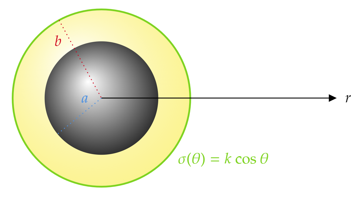
A conducting sphere of radius a, at potential V0, is surrounded by a thin concentric spherical shell of radius b, over which someone has glued a surface charge

σ(θ)=kcos(θ)

Where k is a constant and θ is the usual spherical coordinate.

(a) Find the potential in each region: (i) r>b and (ii) a<r<b. You should find that

V(r,θ)={aV0/r+(b3a3)kcos(θ)/3r2ϵ0rbaV0/r+(r3a3)kcos(θ)/3r2ϵ0arb

(b) Find the induced surface charge σi(θ) on the conductor.

(c) What is the total charge of this system? Check that your answer is consistent with the behavior of V at large r.

Here's the layout of our problem:

Finding the potential

Let's start by recalling that the general solution of Laplace's equation in spherical coordinates (see section 3.3.2: Spherical Coordinates, page 139)

(Eq. 3.65, page 141)V(r,θ)=l=0(Alrl+Blrl+1)Pl(cos(θ))

Where the Pl's are Legendre Polynomials. To keep this solution self-contained, here's a table of them (as seen on page 140):

Where in our case, xcos(θ).

We need to subject Eq. 3.65 to the Boundary conditions that the physical setup has as well as common potential properties.

Outside the sphere of radius b, we must have Al=0 for all l. This is because we need V0 as r. So far this reduces the general solution to

Vrb(r,θ)=Blrl+1Pl(cosθ)

In the yellow region we can't say much for now. To make things clearer, let's denote the solution to the yellow region (arb) with coefficients A and B (rather than A and B as in the outside solution):

Varb(r,θ)=l=0(Alrl+Blrl+1)Pl(cos(θ))

Of course, since the inner sphere is a conductor, we must have:

Vra(r,θ)=V0

Where V0 is constant.

Let's continue imposing constraints and requirements. Recall that potentials must be continuous, meaning that:

Vrb(b,θ)=Varb(b,θ)andVarb(a,θ)=Vra(a,θ)

From continuity at r=b we have:

Vrb(b,θ)=Varb(b,θ)l=0Blbl+1Pl(cosθ)=l=0(Albl+Blbl+1)Pl(cos(θ))(*)Blbl+1=(Albl+Blbl+1)Bl=b2l+1Al+Bl

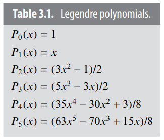
Where the step (*) follows because the Legendre Polynomials are a system of complete and orthogonal polynomials, so the coefficients must match on a 1-to-1 correspondence.

We can see that the continuity at r=b gave us a relation between the unknown coefficients in the outside region and those in the middle region.

From continuity at r=a we have:

Varb(a,θ)=Vra(a,θ)l=0(Alal+Blal+1)Pl(cos(θ))=V0

We can't use the same argument as in the case for continuity at r=b, where we got rid of the Legendre polynomials through a completeness/orthogonality argument, since the right hand side doesn't depend on the Legendre polynomials.

Still, notice the following: The right hand side is a constant. The left hand side is a function of θ. The only way to make these two ideas match is to make the coefficients of all the θ-dependent polynomials zero, and the rest will be equal to the right hand side: V0:

(**)Alal+Blal+1=V0whenl=0(***)Alal+Blal+1=0whenl0

Again, the first Legendre polynomial is the only constant polynomial. From (**) it follows that (we can now change l0):

B0=aV0aA0

And from (***) it follows that

Bl=a2l+1Alwhenl0

At this point, the three potentials can be simplified to (where by simplified we mean having less unknown coefficients):

Vra(r,θ)=V0Varb(r,θ)=l=0(Alrl+Blrl+1)Pl(cos(θ))A0+aV0aA0r+l=1(Alrl+Blrl+1)Pl(cos(θ))Vrb(r,θ)=l=0Blrl+1Pl(cosθ)l=0b2l+1Al+Blrl+1Pl(cosθ)

Let's now impose the condition having to do with σ:

(Eq. 2.36, page 88)VabovenVbelown=1ϵ0σ

Where in this problem

σ=kcos(θ)kP1(cos(θ))Vabove=VrbVbelow=Varb

The fact that σ can be written in terms of one of the Legendre polynomials (with argument cos(θ)) will allow us to generate further constraints. To keep things simple, I will use the potentials without substituting the constraints found through continuity:

Vrbr=l=0Bl(l+1)rl+2Pl(cosθ)Varbr=l=0(Allrl1+Bl(l+1)rl+2)Pl(cosθ)

Equation 2.36 then says:

l=0(Bl(l+1)bl+2Allbl1+Bl(l+1)bl+2)Pl(cosθ)=kϵ0P1(cosθ)

(Notice that I evaluated rb).

If l=1, then:

B12b3A1+B12b3=kϵ0soA1+2b3(B1B1)=kϵ0

Where, as above, we had the match the coefficients of P1 on both sides.

If l1, then the coefficient of Pl must be zero, meaning

Bl(l+1)bl+2Allbl1+Bl(l+1)bl+2=0

Which we further simplify to a more useable form:

(l+1)(BlBl)+lb2l+1Al=0

Let's summarize our findings so far:

(f1) From continuity at r=b:

(i)Bl=b2l+1Al+Bl

(f2) From continuity at r=a:

(ii)B0=aV0aA0(iii)With l0Bl=a2l+1Al

(f3) From surface charge:

(iv)A1+2b3(B1B1)=kϵ0(v)With l1(l+1)(BlBl)+lb2l+1Al=0

Use (ii) and (iii) to write (i) in terms of Al only:

Bl=(b2l+1a2l+1)AlB0=(ba)A0+aV0With l0

Using this and (iii) in (v) for any case where l01:

(l+1)((ba)Al+aV0+a2l+1Al)+lb2l+1Al=0

Since we can factor out Al, it follows that

Al=0

For any l>1. This implies

Bl=0

For any l>1 (were I looked at (iii)). And looking at (i), it follows that

Bl=0

For any l>1. At this point it must be clear that we haven't found any specific values for any of the constants, but we did find that out of the infinite ones we had to find, only 6 might be non-zero: Bl,Al,Bl with l=0 or l=1.

From (v) with l=0 it follows that

B0=B0

And with A0=0, it follows that

B0=B0=aV0

For l=1, it is immediate that

A1=k3ϵ0

Giving (since we can relate A1 and B1):

B1=a3k3ϵ0

Finally:

B1=(b3a3)k3ϵ0

So

V(r,θ)={aV0/r+(b3a3)kcos(θ)/3r2ϵ0rbaV0/r+(r3a3)kcos(θ)/3r2ϵ0arb

Finding the induced surface charge

σinduced(θ)=ϵ0Vr|r=a=ϵ0(2k(r3a3)cos(θ)3ϵr3aV0r2+kcos(θ)ϵ)|r=a=V0ϵ0akcos(θ)

Finding the total charge of the system

qinduced=σinducedda=ϕ=02πθ=02π(V0ϵ0akcos(θ))a2sin(θ)dθdϕ=4πaϵ0V0

Which also corresponds to the total charge of the system.

The behavior of V at large r.

Consider the V for rb. For large r, the 2nd term can be ignored and we are left with

V(r,θ)aV0r

Notice that this is the same as putting the total charge found on part (b) in the point-particle formula.


Back to PHYS405 site