Fernando Garcia

Home     Research     Blog     Other     About me


PHYS405 - Electricity & Magnetism I

Spring 2024

Problem 3.44

Two long straight wires, carrying opposite uniform line charges $\pm \lambda $ are situated on either side of a long conducting cylinder (Fig. 3.39).

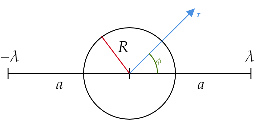
The cylinder (which carries no net charge) has radius $R $, and the wires are a distance $a $ from the axis. Find (to show that) the potential is

\[V(s,\phi )=\frac{\lambda }{4\pi \epsilon _0 }\ln \left\lbrace \frac{(s^2 +a^2 +2sa \cos \left( \phi \right) ) \left[ (sa/R)^2 +R^2 -2sa\cos \left( \phi \right) \right] }{(s^2 +a^2 -2sa\cos \left( \phi \right) ) \left[ (sa/R)^2 +R^2 +2sa\cos \left( \phi \right) \right] } \right\rbrace \]

Here's a dynamic recreation of the original setup:

Since the cylinder is a conductor, it is an equipotential. Suppose this potential is set to $V=0 $. We can use Example 3.2 (page 127) to come up with an analogous configuration with the same boundary conditions. Let's study this example briefly:

We are asked to compute the potential outside a grounded conducting sphere of radius $R $ such that there's a charge $q $ a distance $a $ from its origin. In the solution, due to Lord Kelvin, we see that we can replace the grounded conducting sphere by a point charge with charge

\[q'=\frac{-R}{a}q \]

Situated a distance (between the center of the sphere and the original point charge)

\[b=\frac{R^2 }{a} \]

(Feel free to drag the point $P $ around.)

Now, in Example 3.2 we dealt with a spherical problem. The values for $q' $ and $b $ give, in fact, a spherical surface of equipotential. If instead of point charges we consider line charges, set up as above, we will get cylinders of equipotential. See video below:

Going back to the original problem, we will add two new line charges following Example 3.2's prescription:
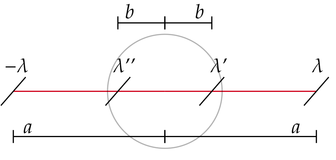
Where

\[b=\frac{R^2 }{a} \]

Let's leave $\lambda ' $ and $\lambda '' $ symbolically for now...

We know that:

\[V(s)=-\frac{1}{4\pi \epsilon _0 }2\lambda \ln \left( \frac{s}{a} \right) \]

(and if you didn't, here's a quick explanation: The $\mathbf{E} $ field of a uniform line charge is $\mathbf{E}=\frac{1}{4\pi \epsilon _0 }\frac{2\lambda }{s}\hat{\mathbf{s}} $. This can be proved using Gauss' law. Then the potential $V(s) $ comes form integrating some reference $s=a $ to $s $.)

With $a $ being some reference $a\neq \infty $. Suppose that the 4 line charges are symmetrically distributed across of axes. That is, a distance $b $ from the origin you will find $\lambda ' $, and a distance $a $ in the same direction you will find $\lambda $, but if you go in the opposite direction you will find $\lambda '' $ and $-\lambda $ at a distance $b $ and $a $, respectively:

To make this easier, let's use laws of logs and rewrite:

\[V(s)=-\frac{1}{4\pi \epsilon _0 }\lambda \ln \left( \frac{s^2 }{a^2 } \right) \]

That is, I used $2\ln (x)=\ln (x^2 ) $. We compute the distances from an arbitrary point on the "$(x,y) $" plane to each of the "origins" for each line charge:

\begin{align*} d_1 ^2 &= (x+a)^2 +y^2 \\ d_2 ^2 &= (x+b)^2 +y^2 \\ d_3 ^2 &= (x-b)^2 +y^2 \\ d_4 ^2 &= (x-a)^2 +y^2 \end{align*}

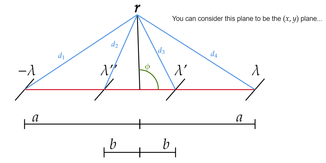
To find those expressions, all I did was vector addition (to avoid thinking about triangles). Before wiring the total potential, let's recall two important log laws:

\begin{align*} \ln (a)+\ln (b) &= \ln (ab) \\ \ln (a)-\ln (b) &= \ln (a/b) \end{align*} With that in mind, we have (by superposition): \begin{align*} V &= V_{-\lambda }+V_{\lambda ''}+V_{\lambda '}+V_{+\lambda } \\ &= \frac{1}{4\pi \epsilon _0 }\bigg(+\lambda \ln \left( \frac{d_1 ^2 }{a_a ^2 } \right) -\lambda '' \ln \left( \frac{d_2 ^2 }{a_b^2 } \right) -\lambda ' \ln \left( \frac{d_3 ^2 }{a_b^2 } \right) -\lambda \ln \left( \frac{d_4 ^2 }{a_a^2 } \right) \bigg)\\ &= \frac{1}{4\pi \epsilon _0 }\bigg( \lambda \ln \frac{d_1 ^2 }{d_4 ^2 } -\lambda '' \ln \left( \frac{d_2 ^2 }{a_b^2 } \right) -\lambda ' \ln \left( \frac{d_3 ^2 }{a_b^2 } \right)\bigg) \end{align*} It seems like we are stuck... What are the values of $\lambda '' $ and $\lambda ' $? Let's try to deduce this using boundary conditions. At the top of the cylinder, we have: \[d_1=d_4 \;\;\;\;\;\;\text{and} \;\;\;\;\;\; d_2 =d_3 \] So \begin{align*} V_{\text{top} }=0 &= \cancel{\lambda \ln (1)}-\lambda '' \ln \left( \frac{d_2 ^2 }{a_b^2 } \right) -\lambda ' \ln \left( \frac{d_3 ^2 }{a_b^2 } \right)\\ &= -\lambda '' \ln \left( \frac{d_2 ^2 }{a_b^2 } \right) -\lambda ' \ln \left( \frac{d_2 ^2 }{a_b^2 } \right) \\ &= -\lambda ''-\lambda ' \end{align*}

So we know that

\[\lambda ''=-\lambda ' \]

A fact that might look trivial, but it's worth obtaining formally.

Let's now consider the two points where "$y=0 $." We find 2 equations:

\begin{align*} 0 &= \lambda \log \left(\frac{(a+R)^2}{(a-R)^2}\right)-\lambda '' \log \left(\frac{(b+R)^2}{a_b^2}\right)-\lambda ' \log \left(\frac{(b-R)^2}{a_b^2}\right) \\ 0 &= \lambda \log \left(\frac{(a-R)^2}{(a+R)^2}\right)-\lambda '' \log \left(\frac{(b-R)^2}{a_b^2}\right)-\lambda ' \log \left(\frac{(b+R)^2}{a_b^2}\right) \end{align*}

Set them equal to each other. Simplify and find:

\[0=\lambda '' \log \left(\frac{(a-R)^2}{(a+R)^2}\right)+\lambda ' \log \left(\frac{(a+R)^2}{(a-R)^2}\right)+\lambda \log \left(\frac{(a+R)^2 (a+R)^2}{(a-R)^2 (a-R)^2}\right) \]

Where I used the fact that $b=R^2 /a $. We know that $\lambda ''=-\lambda ' $, so:

\[0=\lambda '' \log \left(\frac{(a-R)^2}{(a+R)^2}\right)-\lambda '' \log \left(\frac{(a+R)^2}{(a-R)^2}\right)+\lambda \log \left(\frac{(a+R)^2 (a+R)^2}{(a-R)^2 (a-R)^2}\right) \]

Which, after grouping and using log laws, gives:

\[0=\lambda '' \log \left(\frac{(a-R)^2(a-R)^2}{(a+R)^2(a+R)^2}\right)+\lambda \log \left(\frac{(a+R)^2 (a+R)^2}{(a-R)^2 (a-R)^2}\right) \]

Use log laws to induce a (-) sign:

\begin{align*} 0 &= -\lambda '' \log \left( \left[ \frac{(a-R)^2(a-R)^2}{(a+R)^2(a+R)^2} \right] ^{-1} \right)+\lambda \log \left(\frac{(a+R)^2 (a+R)^2}{(a-R)^2 (a-R)^2}\right) \\ &= -\lambda '' \log \left(\frac{(a+R)^2(a+R)^2}{(a-R)^2(a-R)^2}\right)+\lambda \log \left(\frac{(a+R)^2 (a+R)^2}{(a-R)^2 (a-R)^2}\right) \\ &= \log \left(\frac{(a+R)^2(a+R)^2}{(a-R)^2(a-R)^2}\right)(\lambda -\lambda '') \end{align*}

It follows that

\[\lambda =\lambda '' \]

That is:

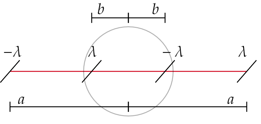
It is important for you to realize that the charge prescription from Example 3.2 doesn't work here!

We can now return to adding the 4 potentials:

\begin{align*} V &= V_{-\lambda }+V_{\lambda ''}+V_{\lambda '}+V_{+\lambda } \\ &= \frac{1}{4\pi \epsilon _0 }\bigg(+\lambda \ln \left( \frac{d_1 ^2 }{a_a ^2 } \right) -\lambda \ln \left( \frac{d_2 ^2 }{a_b^2 } \right) +\lambda \ln \left( \frac{d_3 ^2 }{a_b^2 } \right) -\lambda \ln \left( \frac{d_4 ^2 }{a_a^2 } \right) \bigg)\\ &= \frac{1}{4\pi \epsilon _0 }\lambda \ln \left( \frac{d_1 ^2 d_3 ^2 }{d_2 ^2 d_4 ^2 }\frac{a_a^2 }{a_a^2 }\frac{a_b^2 }{a_b^2 } \right) \\ &= \frac{1}{4\pi \epsilon _0 }\lambda \ln \left( \frac{d_1 ^2 d_3 ^2 }{d_2 ^2 d_4 ^2 } \right)\\ &= \frac{1}{4\pi \epsilon _0 }\lambda \ln \left( \frac{ \left[ (x+a)^2 +y^2 \right] \left[ (x-b)^2 +y^2 \right] }{ \left[ (x+b)^2 +y^2 \right] \left[ (x-a)^2 +y^2 \right] } \right) \end{align*}

We now turn this into cylindrical coordinates, where:

\begin{align*} x &= s \cos \left( \phi \right) \\ y &= s \sin \left( \phi \right) \end{align*}

Noting that:

\begin{align*} \text{From $d_1^2 $:} \;\;\;\; (a+s \cos (\phi ))^2+(s \sin (\phi ))^2 &= a^2+2 a s \cos (\phi )+s^2 \\ \text{From $d_2^2 $:} \;\;\;\; (b+s \cos (\phi ))^2+(s \sin (\phi ))^2 &= b^2+2 b s \cos (\phi )+s^2 \\ &= \frac{a^2 s^2+2 a R^2 s \cos (\phi )+R^4}{a^2}\\ \text{From $d_3^2 $:} \;\;\;\; (-b+s \cos (\phi ))^2+(s \sin (\phi ))^2 &= b^2-2 b s \cos (\phi )+s^2 \\ &= \frac{R^4}{a^2}-\frac{2 R^2 s \cos (\phi )}{a}+s^2\\ \text{From $d_4^2 $:} \;\;\;\; (-a+s \cos (\phi ))^2+(s \sin (\phi ))^2 &= a^2-2 a s \cos (\phi )+s^2 \end{align*}

Which, when plugged into the above expression, give the desired result:

\[V(s,\phi )=\frac{\lambda }{4\pi \epsilon _0 }\ln \left\lbrace \frac{(s^2 +a^2 +2sa \cos \left( \phi \right) ) \left[ (sa/R)^2 +R^2 -2sa\cos \left( \phi \right) \right] }{(s^2 +a^2 -2sa\cos \left( \phi \right) ) \left[ (sa/R)^2 +R^2 +2sa\cos \left( \phi \right) \right] } \right\rbrace \]

Here's a cross-section, at some $z $, of the potential:

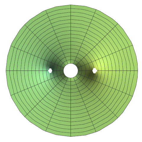
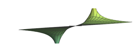
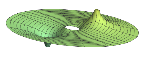
The middle hole represents the inside of the cylinder. We can't use the method of images to find the potential there as we added new charges in that area.

The outer 2 holes represent the positions of the line charges.


Back to PHYS405 site