Fernando Garcia
Home Research Blog Other About me
PHYS405 - Electricity & Magnetism I
Spring 2024
Problem 3.13
Two semi-infinite grounded conducting planes meet at right angles. In the region between them, there is a point charge
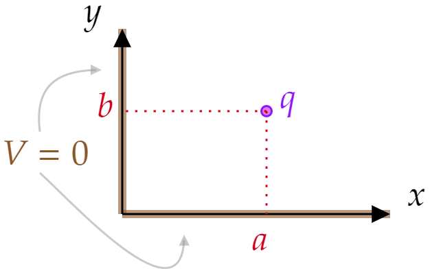
What charges do you need, and where should they be located?
What is the force on
How much work did it take to bring
Suppose the planes met at some angler other than 90 degrees. Would you still be able to solve the problem by the method of images? If not, for what particular angles does the method work?
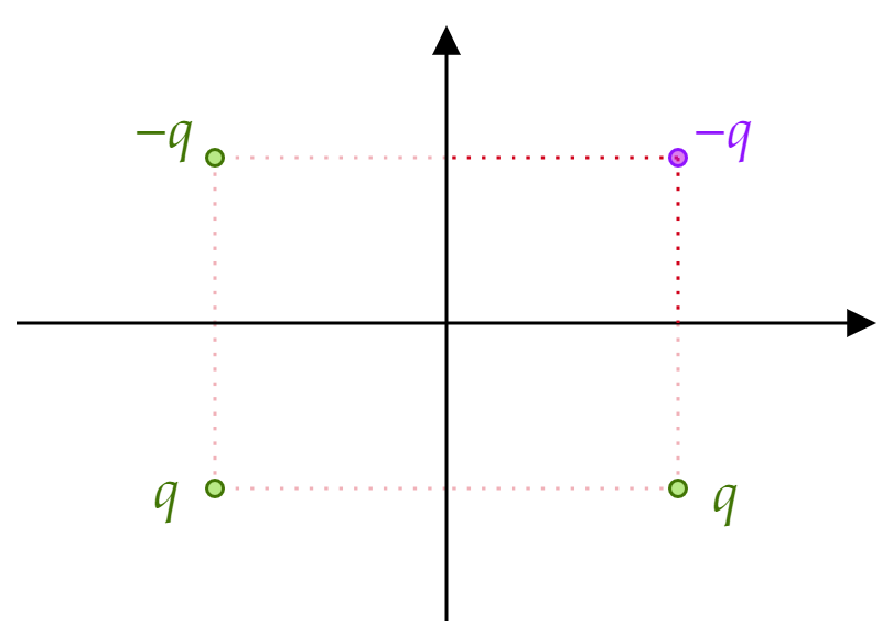
We have to place image charges in such a way that we can replicate the boundary conditions.
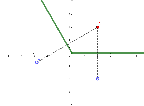
Let's start by formalizing where
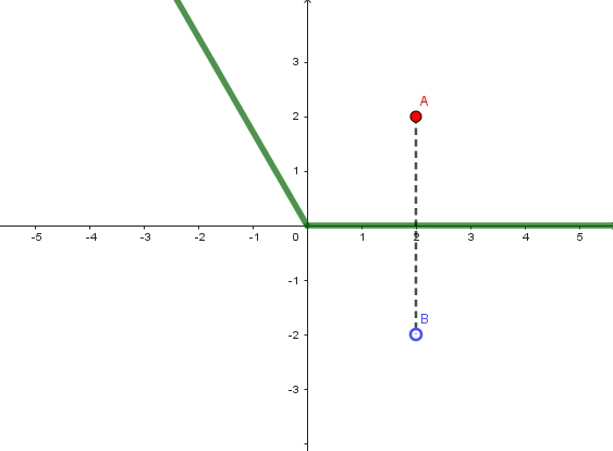
To achieve the first, we can place a
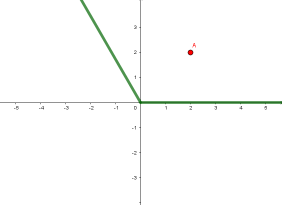
Notice how the potential (red surface) is 0 on the axes:
Because of the first uniqueness theorem (see page 119 of your book), it follows that the potential of the dual semi-infinite plane and charge
The force on
The work can be calculated using the image configuration. Recall from chapter 2 that:
Where the potential will be the potential from the 3 image charges:
Which evaluated at
So
To see at what other angles this would work, go look at the plot of the potential again (red surface above). We see that we created 4 regions that behave quite similarly. This is precisely the key to answer this: we need to divide the plane in equal sections, and to do this the angle has to be an (integer) divisor of 180 degrees.
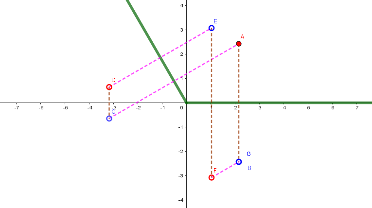
Other angles won't work as they will require us to add image charges inside the region we are interested in studying. Consider, for instance, 120 degrees. This is an enlightening example, as it divides 360 (not 180, though, which is what we are really interested in):
Place a charge anywhere in the area of interest, and consider the 2 grounded semi-planes:
To have
To have
 But after we added
 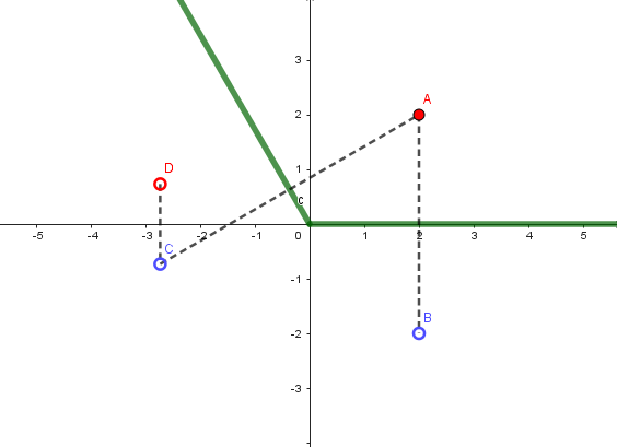 But after we added
 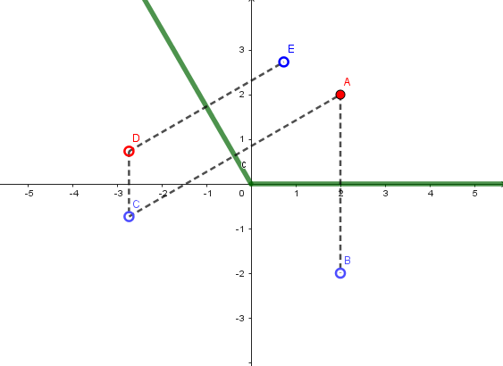 There are 2 issues here, the second more important than the first:
(1) It is clear that we will need to add yet another charge (reflecting
(2) We placed a charge inside the region of interest. That is, we have a different problem and this no longer represents the initial configuration.
Extra: The answer to whether the sequence of reflections ever converges is that, yes:
We reflect