---

Fernando Garcia

Home     Research     Blog     Other     About me

---

Brute forcing Feynman diagrams: Combinations and symmetry factors

July 12th, 2024.

Introduction

Feynman diagrams are such an important concept (and tool!) that even many of those who have never worked with Quantum Field Theory know about their existence.

To recapitulate, Feynman diagrams appear from expanding a theory into a series (to be precise, from expanding the interacting partition function into a series). They are a visual representation of a given term in the expansion.

These connection between terms of a series and the diagrams allows us to classify them by the amount of external points (sources) $E$, vertices $V$, and propagators (curve segment) $P$.

This blog post will focus on ${\varphi }^3$ theory, where $E$, $V$, and $P$ are related by

$$E=2P-3V$$

Things start to get a bit out of control when we realize that for a given $P$ and $V$, there are many, many terms in the expansion. It is then relevant to realize how many terms in the expansion give the same Feynman diagram.

This is known as the symmetry factor. It can be calculated quickly and easily for simple diagrams, but sometimes counting gets complicated or tedious. Let's explore a brute-force way get this number.

In ${\varphi }^3$ theory, $Z_1(J)$ takes the form (see Srednicki)

$$Z_1(J)\propto \sum _{V=0}^{\mathrm{\infty }}\frac{1}{V!}{[\frac{i{Z}_{g}g}{6}\int d^{4}x{\left(\frac{1}{i}\frac{\delta }{\delta J(x)}\right)}^3]}^V\times \sum _{P=0}^{\mathrm{\infty }}\frac{1}{P!}{[\frac{i}{2}\int d^{4}y{d}^{4}zJ(y)\mathrm{\Delta }(y-z)J(z)]}^p$$

Warning: This method is by no means ideal/fast. The purpose of this post is to show how all the numbers are connected.

Terms with $E=0$, $V=2$ (therefore $P=3$).

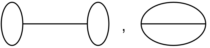
If we have two vertices, each has to have 3 lines coming in/out of it, and there are 3 lines to place on the diagram, it is clear that there are only two possible Feynman diagrams:

We start by noting that the term with $V=2$ and $P=3$ (in $Z_1$) gives a numerical factor of

$$\frac{1}{2^P{6}^V(V!)(P!)}{|}_{V=2,P=3}=\frac{1}{3456}$$

This number will be important in a second. Now notice that we have 6 functional derivatives (with respect to sources $J(x)$) acting on a product of 6 sources. Carrying out the product rule will yield

$$6!=720\text{terms}$$

That is, there are 720 diagrams to be considered. Are they all different? How many are the same? As speculated above, we hope to get only 2 diagrams.

To keep track of variables, let's use the following variables:

$$\frac{1}{3456}\int d^{4}x{d}^{4}w{d}^4{y}_1{d}^4{y}_2{d}^4{y}_3{d}^4{z}_1{d}^4{z}_2{d}^4{z}_3{\left(\frac{1}{i}\frac{\delta }{\delta J(x)}\right)}^3{\left(\frac{1}{i}\frac{\delta }{\delta J(w)}\right)}^{3}J(y_1)\mathrm{\Delta }(y_1-z_1)J(z_1)J(y_2)\mathrm{\Delta }(y_2-z_2)J(z_2)J(y_3)\mathrm{\Delta }(y_3-z_3)J(z_3)$$

So we will have a product of three propagators $\mathrm{\Delta }(y_1-z_1)\mathrm{\Delta }(y_2-z_2)\mathrm{\Delta }(y_3-z_3)$ times 720 terms. Each one of the terms is of the form

$$\delta (x-)\delta (x-)\delta (x-)\delta (w-)\delta (w-)\delta (w-)$$

Where the spaces are to be filled with (once each) $y_1,y_2,y_3,z_1,z_2,z_3$. For instance:

$$\mathrm{\Delta }(y_1-z_1)\mathrm{\Delta }(y_2-z_2)\mathrm{\Delta }(y_3-z_3)(\delta (x-y_1)\delta (x-y_2)\delta (x-y_3)\delta (w-z_1)\delta (w-z_2)\delta (w-z_3)+\text{the other 719 terms})$$

It is clear that we can compute the six $\int d^4{y}_1{d}^4{y}_2{d}^4{y}_3{d}^4{z}_1{d}^4{z}_2{d}^4{z}_3$ integrals, which will turn the 3 propagatos into propagators in terms of $x$s and $w$s.

There are only two possible cases, we end up (after computing the integrals over the deltas) with $\mathrm{\Delta }(x-w{)}^3$, or $\mathrm{\Delta }(0{)}^2\mathrm{\Delta }(x-y)$. Notice how there is simply no way to get $\mathrm{\Delta }(0{)}^3$ out of the available variables, the same goes for $\mathrm{\Delta }(0)\mathrm{\Delta }(x-w{)}^2$.

For the case $\mathrm{\Delta }(x-w{)}^3$, let's see how many terms we have (out of the 720). There are 6 ways to place a given $y_i$ among the 6 half-filled deltas. If we picked one with an $x$, then we must place $z_i$ in one of the 3 deltas with $w$ (and vice versa).

Now pick $y_j$ for $i\ne j$. There are 4 half-filled deltas to pick. This forces us to place $z_j$ in one of the remaining 2 deltas with the opposite $x/w$ variable.

Finally, we can place $y_k$ for $i\ne j\ne k$ in either of the 2 remaining deltas, and the last $z_k$ variable gets placed in the remaining delta with opposite variable.

In total, we have

$$6\times 3\times 4\times 2\times 2=288\text{terms}$$

They all, of course, represent the same diagram:

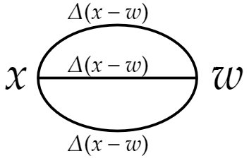
We are pretty sure that there should only be an additional diagram, corresponding to terms of the form $\mathrm{\Delta }(x-y)\mathrm{\Delta }(0{)}^2$. We could right away say that there are $720-288=432$ such terms. Instead, let's work out the combinations and see that it is truly 432 (and we can finally confirm that there are 2 two diagrams, since we would then have 720 worked out terms).

We can place $y_i$ in any of the deltas: 6.

To induce a $\mathrm{\Delta }(0)$, we place another $y_j$ in any of the two remaining deltas with the same variable: 2.

To induce another $\mathrm{\Delta }(0)$, we place any of the $z_i$ in any of the 3 deltas with the other variable: 9 ways.

The $\mathrm{\Delta }(0)$ happens once we place yet another $z_j$ in any of the two remaining deltas with the other variable: 2 ways.

There are 2 ways to place the remaining $y_k,z_k$ in the two last deltas. We see that:

$$6\times 2\times 9\times 2\times 2=432\text{terms}$$

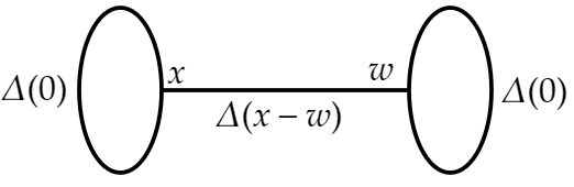
As expected. Those terms represent the diagram:

Contributions and symmetry factors

We must not forget that we still have the $\int d^{4}x{d}^{4}w$ integrals over the above expressions. Furthermore, the numerical factor of $1/3456$ combines with the amount of terms for the same diagram to give the proper symmetry factor:

$$\begin{array}{rl}\frac{1}{3456}\cdot 288& =\frac{1}{12}\\ \frac{1}{3456}\cdot 432& =\frac{1}{8}\end{array}$$

In this post we are not interested in computing corrections or observables, but if we want to, we must also remember the factors of $g$, $Z_g$, and any other constants in the expansion of the path integral.

It is also relevant to note that we got the exact same expressions as if we had followed the rules of adding $\frac{1}{i}\mathrm{\Delta }(x-y)$ per propagator, and $i{Z}_{g}g\int d^{4}x$ per vertex.

Terms with $E=1$, $V=1$ (therefore $P=2$).

It is clear that there is only one diagram for this scenario:

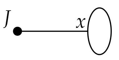
Where the black filled dot is now representing a source/external point.

We get a numerical factor of

$$\frac{1}{2^P{6}^V(V!)(P!)}{|}_{V=1,P=2}=\frac{1}{48}$$

in the expansion, as well as the integral (again, brushing off the factors of $i,g,Z_g$, and the numerical factor of $1/48$ for now):

$$\int d^{4}x{d}^4{y}_1{d}^4{y}_2{d}^4{z}_1{d}^4{z}_2\frac{\delta }{\delta J(x)}\frac{\delta }{\delta J(x)}\frac{\delta }{\delta J(x)}J(y_1)\mathrm{\Delta }(y_1-z_1)J(z_1)J(y_2)\mathrm{\Delta }(y_2-z_2)J(z_2)$$

Which, when acting with the functional derivatives, we find:

$$\int d^{4}x{d}^4{y}_1{d}^4{y}_2{d}^4{z}_1{d}^4{z}_2\mathrm{\Delta }(y_1-z_1)\mathrm{\Delta }(y_2-z_2)(\text{terms of the form}J()\delta (x-)\delta (x-)\delta (x-))$$

The first question is: how many terms are there? A careful analysis shows that we get $4\times 3\times 2=24$ terms. It is also to see that they are all of the same form. Either the two $y$s will get placed in $\delta$s and the $z$s one in a delta and one inside the source $J$, or vice versa.

After computing the $d^4{y}_1{d}^4{y}_2{d}^4{z}_1{d}^4{z}_2$ integrals, we find:

$$\int d^{4}x{d}^4{y}_{1}J(y_1)\mathrm{\Delta }(y_1-x)\mathrm{\Delta }(0)$$

Which is what the rules (times constant factors) dictate (for each source, add the integral $i\int d^{4}yJ(y)$).

Since we only have 1 diagram and 24 terms, we invoke the numerical factor of $1/48$ to see that the symmetry factor of the diagram is:

$$\frac{1}{48}\cdot 24=\frac{1}{2}$$

As expected.

Final remarks and conclusion

It is clear that Feynman diagrams are based on solid ground. The above analysis can get complicated even for the simplest of conditions ($P,V$). More than a tool, doing the above is instructive while studying Quantum Field Theory. It is one of those things you do once and never come back to it, but the implications stay with you for the rest of your life.

I think turning this into a computer program shouldn't be too complicated. By coding the rules of functional differentiation, one could possibly avoid having to do a combinatorics-heavy analysis.

Picture Credits: Jorge Cham, phdcomics.

Back to Blogs