---

Fernando Garcia

Home     Research     Blog     Other     About me

---

Complex scalar fields: Mode expansions and quantization

July 10th, 2024.

Introduction

The basics of (real) scalar field theory and its quantization are heavily covered in various books and review articles. Brief comments are usually made on its complex brother: field theory of a complex scalar field.

In this blog post I will be going over, in detail, the basics of having a complex scalar field and its quantization. A final comment will be made on the ground state of the theory. This post was heavily inspired by a Problem in Mark Srednicki's QFT book.

As a classical field

Let's make the theory concrete by writing down the its Lagrangian:

$$\mathcal{L}=-{\partial }^{\mu }{\varphi }^{†}{\partial }_{\mu }\varphi -m^2{\varphi }^{†}\varphi +{\mathrm{\Omega }}_0$$

Where ${\mathrm{\Omega }}_0$ is a constant. The equation of motion of a real scalar field analogous to the one above is the Klein-Gordon equation. It is straight forward to show that both $\varphi$ and ${\varphi }^{†}$ follow the same equation.

If we plug the Lagrangian into the Euler-Lagrange equation for the $\varphi$ field, we find:

$$\begin{array}{rl}\frac{\partial \mathcal{L}}{\partial \varphi }& ={\partial }_{\mu }\left(\frac{\partial \mathcal{L}}{\partial ({\partial }_{\mu }\varphi )}\right)\\ -m^2{\varphi }^{†}& ={\partial }_{\mu }(-{\partial }^{\mu }{\varphi }^{†})\\ {\partial }_{\mu }{\partial }^{\mu }{\varphi }^{†}-m^2{\varphi }^{†}& =0\\ ({\partial }_{\mu }{\partial }^{\mu }-m^2){\varphi }^{†}& =0\end{array}$$

And if we do it for the ${\varphi }^{†}$ field, we find:

$$\begin{array}{rl}\frac{\partial \mathcal{L}}{\partial {\varphi }^{†}}& ={\partial }_{\mu }\left(\frac{\partial \mathcal{L}}{\partial ({\partial }_{\mu }{\varphi }^{†})}\right)\\ -m^2\varphi & ={\partial }_{\mu }(-{\partial }^{\mu }\varphi )\\ {\partial }_{\mu }{\partial }^{\mu }\varphi -m^2\varphi & =0\\ ({\partial }_{\mu }{\partial }^{\mu }-m^2)\varphi & =0\end{array}$$

Where it is relevant to remark that we treat $\varphi$ and ${\varphi }^{†}$ as independent fields. From a canonical point of view (to be worked out later on), the Hamiltonian (density) plays a central role, and as such we need to find the canonical momenta of the theory. We see that

$$\begin{array}{rl}{\mathrm{\Pi }}_{\varphi }(x)& =\frac{\partial \mathcal{L}}{\partial \dot{\varphi }}\\ & ={\dot{\varphi }}^{†}(x)\end{array}$$

And

$$\begin{array}{rl}{\mathrm{\Pi }}_{{\varphi }^{†}}(x)& =\frac{\partial \mathcal{L}}{\partial {\dot{\varphi }}^{†}}\\ & =\dot{\varphi }(x)\end{array}$$

So the Hamiltonian (density) reads:

$$\begin{array}{rl}\mathcal{H}& ={\mathrm{\Pi }}_{\varphi }\dot{\varphi }+{\mathrm{\Pi }}_{{\varphi }^{†}}{\dot{\varphi }}^{†}-\mathcal{L}\\ & ={\dot{\varphi }}^{†}\dot{\varphi }+\dot{\varphi }{\dot{\varphi }}^{†}+{\partial }^{\mu }{\varphi }^{†}{\partial }_{\mu }\varphi +m^2{\varphi }^{†}\varphi -{\mathrm{\Omega }}_0\\ & ={\dot{\varphi }}^{†}\dot{\varphi }+\dot{\varphi }{\dot{\varphi }}^{†}+{\eta }^{\mu \nu }{\partial }_{\mu }{\varphi }^{†}{\partial }_{\mu }\varphi +m^2{\varphi }^{†}\varphi -{\mathrm{\Omega }}_0\\ & ={\dot{\varphi }}^{†}\dot{\varphi }+\dot{\varphi }{\dot{\varphi }}^{†}+(-{\dot{\varphi }}^{†}\dot{\varphi }+\mathrm{\nabla }{\varphi }^{†}\mathrm{\nabla }\varphi )+m^2{\varphi }^{†}\varphi -{\mathrm{\Omega }}_0\\ & ={\mathrm{\Pi }}_{{\varphi }^{†}}{\mathrm{\Pi }}_{\varphi }+\mathrm{\nabla }{\varphi }^{†}\mathrm{\nabla }\varphi +m^2{\varphi }^{†}\varphi -{\mathrm{\Omega }}_0\end{array}$$

Now, let's suppose we expand $\varphi$ in terms of modes:

$$\varphi (x)=\int \widetilde{dk}(a(\mathbf{k})e^{ikx}+b^{†}(\mathbf{k})e^{-ikx})$$

Where

$$\widetilde{dk}=\frac{d^{3}k}{(2\pi {)}^{3}2\omega }$$

It is relevant to remark that $kx\equiv \mathbf{k}\cdot \mathbf{x}-\omega t$. That is, we should not forget the fact that there's a time-dependent exponential factor (even though the integral (measure) only goes over spatial momentum modes).

The immediate question is what are $a(\mathbf{k})$ and $b^{†}(\mathbf{k})$ (that is, how are they related to the field itself?). Here it is good to note that in the case that $\varphi$ is a real field, $a$ and $b$ are directly related to each other (in fact, we can show that ${\varphi }^{\ast }(x)=\varphi (x)$ implies $b^{\ast }(-\mathbf{k})=a(\mathbf{k})$) and we get the familiar expressions. The simplification is not as simple for the case of a complex $\varphi$ field, but we can work it out.

Recall the important identity:

$$\int d^{3}x{e}^{i\mathbf{q}\cdot \mathbf{x}}=(2\pi {)}^3{\delta }^3(\mathbf{q})$$

We can apply it on both sides of the mode expansion, that is, let's multiply by $e^{iq\cdot x}$ and then integrate spatially. Notice again that we are adding an exponential with both time and spatial components. Performing the aforementioned steps will induce some deltas in the integrand which will allow us to chug down the momentum integrals nicely:

$$\begin{array}{rl}\varphi (x)& =\int \widetilde{dk}(a(\mathbf{k})e^{ikx}+b^{†}(\mathbf{k})e^{-ikx})\\ e^{iqx}\varphi (x)& =e^{iqx}\int \widetilde{dk}(a(\mathbf{k})e^{ikx}+b^{†}(\mathbf{k})e^{-ikx})\\ e^{iqx}\varphi (x)& =e^{i(\mathbf{q}\cdot \mathbf{x}-\alpha t)}\int \widetilde{dk}(a(\mathbf{k})e^{ikx}+b^{†}(\mathbf{k})e^{-ikx})\\ e^{iqx}\varphi (x)& =\int \widetilde{dk}(a(\mathbf{k})e^{i\mathbf{k}\cdot \mathbf{x}+i\mathbf{q}\cdot \mathbf{x}-i\omega t-i\alpha t}+b^{†}(\mathbf{k})e^{-i\mathbf{k}\cdot \mathbf{x}+i\mathbf{q}\cdot \mathbf{x}+i\omega t-i\alpha t})\\ \int d^{3}x{e}^{iqx}\varphi (x)& =\int \widetilde{dk}{d}^{3}x(a(\mathbf{k})e^{i\mathbf{k}\cdot \mathbf{x}+i\mathbf{q}\cdot \mathbf{x}-i\omega t-i\alpha t}+b^{†}(\mathbf{k})e^{-i\mathbf{k}\cdot \mathbf{x}+i\mathbf{q}\cdot \mathbf{x}+i\omega t-i\alpha t})\\ \int d^{3}x{e}^{iqx}\varphi (x)& =\int \widetilde{dk}{d}^{3}x(a(\mathbf{k})e^{i(\mathbf{k}+\mathbf{q})\cdot \mathbf{x}}{e}^{-i(\omega +\alpha )t}+b^{†}(\mathbf{k})e^{i(\mathbf{q}-\mathbf{k})\cdot \mathbf{x}}{e}^{+i(\omega -\alpha )t})\\ & =\int \widetilde{dk}(a(\mathbf{k})(2\pi {)}^3{\delta }^3(\mathbf{k}+\mathbf{q})e^{-i(\omega +\alpha )t}+b^{†}(\mathbf{k})(2\pi {)}^3{\delta }^3(\mathbf{q}-\mathbf{k})e^{+i(\omega -\alpha )t})\\ & =\frac{1}{2\omega }(a(-\mathbf{q})e^{-i(\omega +\alpha )t}+b^{†}(\mathbf{q})e^{+i(\omega -\alpha )t})\end{array}$$

We have made good progress so far. To further simplify, we need to deal with $\omega$ and $\alpha$. We first note that they are the temporal parts of $k$ and $q$, respectively. Since $k$ and $q$ have equal magnitudes and equal spatial parts, we must have that the temporal parts are equal to each other, that is:

$$\omega =\alpha$$

In the above I will substitute $\mathbf{q}\to -\mathbf{q}$ (where terms with $\alpha$ pick up a negative sign) to get:

$$\begin{array}{rl}\int d^{3}x{e}^{-iqx}\varphi (x)& =\frac{1}{2\omega }(a(\mathbf{q})e^{-i(\omega -\alpha )t}+b^{†}(-\mathbf{q})e^{+i(\omega +\alpha )t})\\ & =\frac{1}{2\omega }(a(\mathbf{q})e^{-i(\alpha -\alpha )t}+b^{†}(-\mathbf{q})e^{+i(\alpha +\alpha )t})\\ & =\frac{1}{2\alpha }(a(\mathbf{q})+b^{†}(-\mathbf{q})e^{+i2\alpha t})\end{array}$$

Now, I will follow the trick Srednicki used to get another linear combination that's not parallel to the above one. If we consider instead expanding ${\partial }_0\varphi$ into momentum modes:

$$\begin{array}{rl}{\partial }_0(\varphi (x))& ={\partial }_0[\int \widetilde{dk}(a(\mathbf{k})e^{ikx}+b^{†}(\mathbf{k})e^{-ikx})]\\ & =\int \widetilde{dk}((-i\omega )a(\mathbf{k})e^{ikx}+(+i\omega )b^{†}(\mathbf{k})e^{-ikx})\end{array}$$

We pick up factors ($\pm$: negative for the first one and positive for the second term because $kx\equiv \mathbf{k}\cdot \mathbf{x}-\omega t$) of $i\omega$ and the rest follows in the same way. It is then clear that:

$$\begin{array}{rl}\int d^{3}x{e}^{-iqx}{\partial }_0\varphi (x)& =\frac{1}{2\alpha }((-i\omega )a(\mathbf{q})+(+i\omega )b^{†}(-\mathbf{q})e^{+i2\alpha t})\\ & =\frac{1}{2\alpha }((-i\alpha )a(\mathbf{q})+(i\alpha )b^{†}(-\mathbf{q})e^{+i2\alpha t})\\ & =\frac{i}{2}(-a(\mathbf{q})+b^{†}(-\mathbf{q})e^{+i2\alpha t})\end{array}$$

At this point we have a system of equations. One can right away find solutions to $a(\mathbf{q})$:

$$a(\mathbf{q})=\int d^{3}x{e}^{-iqx}(\alpha \varphi (x)+i{\mathrm{\Pi }}_{{\varphi }^{†}}(x))$$

And we can find a solution to $b^{†}(-\mathbf{q})$ (and thus $b(-\mathbf{q})$, once we undo the dagger). How do we find $b(\mathbf{q})$ from it? There is a connection/relation between the complex field and $a/b$. If we replace $\varphi$ by ${\varphi }^{†}$ in the mode expansion, we see that the roles of $a$ and $b$ get interchanged. As such, $b(\mathbf{q})$ is given by substituting $\varphi$ for ${\varphi }^{†}$ in $a(\mathbf{q})$:

$$b(\mathbf{q})=\int d^{3}x{e}^{-iqx}(\alpha {\varphi }^{†}(x)+i{\mathrm{\Pi }}_{\varphi }(x))$$

Where I used the fact that ${\mathrm{\Pi }}_{\varphi }={\partial }_0{\varphi }^{†}$ and ${\mathrm{\Pi }}_{{\varphi }^{†}}={\partial }_0\varphi$. To make the equations easier to read, let's go back to writing (this is a simple relabeling of variables) $q\to k=(\omega ,\mathbf{k})$:

$$\begin{array}{rl}a(\mathbf{k})& =\int d^{3}x{e}^{-ikx}(\omega \varphi (x)+i{\mathrm{\Pi }}_{{\varphi }^{†}}(x))\\ b(\mathbf{k})& =\int d^{3}x{e}^{-ikx}(\omega {\varphi }^{†}(x)+i{\mathrm{\Pi }}_{\varphi }(x))\end{array}$$

As a quantum field

Having written down $a(\mathbf{k})$ and $b(\mathbf{k})$, we can start to talk about the field as a quantum field. That is, let's impose canonical commutation relations on the fields (and the respective momenta):

$$\begin{array}{rl}[\varphi (\mathbf{x},t),\varphi (\mathbf{y},t)]& =0\\ [{\varphi }^{†}(\mathbf{x},t),{\varphi }^{†}(\mathbf{y},t)]& =0\\ [\varphi (\mathbf{x},t),{\mathrm{\Pi }}_{{\varphi }^{†}}(\mathbf{y},t)]& =0\\ [{\varphi }^{†}(\mathbf{x},t),{\mathrm{\Pi }}_{\varphi }(\mathbf{y},t)]& =0\\ [\varphi (\mathbf{x},t),{\mathrm{\Pi }}_{\varphi }(\mathbf{y},t)]& =i{\delta }^3(\mathbf{x}-\mathbf{y})\\ [{\varphi }^{†}(\mathbf{x},t),{\mathrm{\Pi }}_{{\varphi }^{†}}(\mathbf{y},t)]& =i{\delta }^3(\mathbf{x}-\mathbf{y})\\ [{\mathrm{\Pi }}_{\varphi }(\mathbf{x},t),{\mathrm{\Pi }}_{\varphi }(\mathbf{y},t)]& =0\\ [{\mathrm{\Pi }}_{{\varphi }^{†}}(\mathbf{x},t),{\mathrm{\Pi }}_{{\varphi }^{†}}(\mathbf{y},t)]& =0\\ [{\mathrm{\Pi }}_{\varphi }(\mathbf{x},t),{\mathrm{\Pi }}_{{\varphi }^{†}}(\mathbf{y},t)]& =0\end{array}$$

Visually, let's introduce the table:

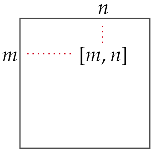
A particular feature of it is that it highlights the antisymmetric nature of the current problem. In fact, out of the 16 combinations, we only really need to formally compute, at most, 10. Others might follow from already computed results. For the case of the field variables:

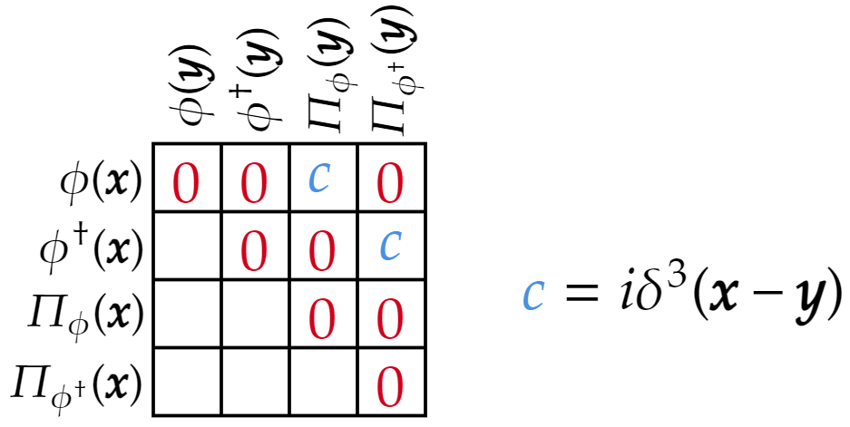
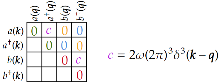
We now ask, what are the commutation relations for $a(\mathbf{k})$ and $b(\mathbf{k})$? Here are the results

And we now justify them. We notice that some the zeros were color-coded. This signifies that the result of one of them directly implies that of another of the same color.

The first commutator, $[a,a]$, is quite trivial. As demonstrated above, $a(\mathbf{k})$ depends on the field $\varphi$ and the conjugate momenta of its complex conjugate ${\mathrm{\Pi }}_{{\varphi }^{†}}$. As such, all the commutators are between the same object or between distinct objects for the un-daggered/daggered components. As such, it vanishes. And

$$[a,a]=0\Rightarrow [a^{†},a^{†}]=0$$

The exact same argument follows for $[b,b]=0$, further:

$$[b,b]=0\Rightarrow [b^{†},b^{†}]=0$$

So far 4 commutators. To continue, let's recall that

$$[A+B,C]=[A,C]+[B,C]$$

So

$$\begin{array}{rl}[A+B,C+D]& =[A,C+D]+[B,C+D]\\ & =[A,C]+[A,D]+[B,C]+[B,D]\end{array}$$

Let's now compute the orange $0$s.

Consider $[a,b]$. Within the integrand, the non-zero commutators are

$$\begin{array}{rl}[\varphi (x),\mathrm{\Pi }(y)]+{[\varphi (y),\mathrm{\Pi }(x)]}^{†}& =i{\delta }^3(\mathbf{x}-\mathbf{y})+(i{\delta }^3(\mathbf{x}-\mathbf{y}){)}^{†}\\ & =i{\delta }^3(\mathbf{x}-\mathbf{y})-i{\delta }^3(\mathbf{x}-\mathbf{y})\\ & =0\end{array}$$

So

$$[a,b]=0$$

And we notice that

$$[a,b]=0\Rightarrow [a^{†},b^{†}]=0$$

To compute the blue $0$s, it is enough to see the expansions of $a$ and $b^{†}$. Both of them contain the field $\varphi$ and the momenta of the field ${\varphi }^{†}$. It is clear that all the commutators go to zero, and thus

$$[a,b^{†}]=0$$

So

$$[a,b^{†}]=0\Rightarrow [a^{†},b]=0$$

Let's finalize by working out the non-zero commutators.

$$\begin{array}{rl}[a(\mathbf{k}),a^{†}(\mathbf{q})]& =[\int d^{3}x{e}^{-ikx}\{\omega \varphi (x)+i{\mathrm{\Pi }}_{{\varphi }^{†}}(\mathbf{x})\},\int d^{3}y{e}^{+iqy}\{\omega {\varphi }^{†}(y)-i{\mathrm{\Pi }}_{\varphi }(y)\}]\\ & =\int d^{3}x{d}^{3}y{e}^{+iqy-ikx}[\omega \varphi (x)+i{\mathrm{\Pi }}_{{\varphi }^{†}}(x),\omega {\varphi }^{†}(y)-i{\mathrm{\Pi }}_{\varphi }(y)]\\ & =\int d^{3}x{d}^{3}y{e}^{+iqy-ikx}({\omega }^2\cancel{[\varphi (x),\varphi (y)]}-i\omega [\varphi (x),{\mathrm{\Pi }}_{\varphi }(y)]+i\omega [{\mathrm{\Pi }}_{{\varphi }^{†}}(x),{\varphi }^{†}(y)]-i^2\cancel{[{\mathrm{\Pi }}_{{\varphi }^{†}}(x),{\mathrm{\Pi }}_{\varphi }(y)]})\\ & =\int d^{3}x{d}^{3}y{e}^{+iqy-ikx}(-2i\omega )[\varphi (x),{\mathrm{\Pi }}_{\varphi }(y)]\\ & =\int d^{3}x{d}^{3}y{e}^{+iqy-ikx}(-2i\omega )i{\delta }^3(\mathbf{x}-\mathbf{y})\\ & =2\omega \int d^{3}x{d}^{3}y{e}^{+iqy-ikx}{\delta }^3(\mathbf{x}-\mathbf{y})\\ & =2\omega \int d^{3}x{e}^{+iqx-ikx}\\ & =2\omega \int d^{3}x{e}^{-(k-q)x}\\ & =2\omega (2\pi {)}^3{\delta }^3(\mathbf{k}-\mathbf{q})\end{array}$$

As proposed.

Concluding remarks and the Hamiltonian

The model above is indeed instructive and worth working out. To keep this blog post short, I won't be showing all the steps in regards to getting a Hamiltonian in terms of $a$s and $b$s. I will give an overview of the result and in a later blog we can work things out step by step.

To compare, we recall that the Hamiltonian of a single real scalar field $\phi$ is given by:

$$H=\int \widetilde{dk}\omega a^{†}(\mathbf{k})a(\mathbf{k})+({\mathcal{E}}_0-{\mathrm{\Omega }}_0)V$$

Where ${\mathcal{E}}_0$ represents the total zero-point energy of all the oscillators, per unit volume. It is here where we find our first infinity when studying QFT. Such an integral diverges. We could introduce an ultraviolet cutoff $\mathrm{\Lambda }$, or give a value to ${\mathrm{\Omega }}_0$ to get rid of it. In the case of the real field, we simply let ${\mathrm{\Omega }}_0={\mathcal{E}}_0$.

If we now turn our attention towards the complex field $\varphi ,{\varphi }^{†}$, we can show that the Hamiltonian presented earlier in the blog post can be written as

$$H=(2{\mathcal{E}}_0-{\mathrm{\Omega }}_0)V+\int \widetilde{dk}\omega [a^{†}(\mathbf{k})a(\mathbf{k})+b^{†}(\mathbf{k})b(\mathbf{k})]$$

In such a case, it is clear that the infinity issue gets fixed by setting ${\mathrm{\Omega }}_0=2{\mathcal{E}}_0$. It must be said that this sets the ground state energy to zero.

Back to Blogs